validation_tests • childpen

Overview

The aim of this vignette is show how to perform correct validation tests using closest-not-yet-treated control groups using childpen.

Simulate data

The package has a built in simulation function to draw data resembling child penalty studies.

library(childpen)

N <- 20000
data <- simulate_data(n_individuals = N)
data |> tibble()
#> # A tibble: 420,000 × 6
#>       id female   age     D   Y_inf       Y
#>    <int>  <int> <int> <int>   <dbl>   <dbl>
#>  1     1      1    20    37   4455.   4455.
#>  2     1      1    21    37   7057.   7057.
#>  3     1      1    22    37  15138.  15138.
#>  4     1      1    23    37  31188.  31188.
#>  5     1      1    24    37  26199.  26199.
#>  6     1      1    25    37  45635.  45635.
#>  7     1      1    26    37  46719.  46719.
#>  8     1      1    27    37  39892.  39892.
#>  9     1      1    28    37 127141. 127141.
#> 10     1      1    29    37 109342. 109342.
#> # ℹ 419,990 more rows

The correct validation tests

See the DID vignette (link) for an explainer on the $2\times2$ comparisons in childpen. Recall that $d$ is the treatment group, $a$ is the target age, and $d^\prime=a+1$ is the closest not-yet-treated control group.

Assume that when presenting results, post-treatment, you report estimates for event times $e=0,...,5$ . Then, for each treatment group $d$ you use 6 different control groups in post-treatment estimation. As the identification assumptions (e.g., parallel trends for DID) must hold for each point-estimate separately, this implies that it must hold within each treatment-control pair.

The above argument means that the validation tests should be done separately by treatment-control combinations. Returning to the above example, if you want to show results for $e=0,...,5$ then you need to conduct pre-trend analysis for 6 different control groups. This is done automatically in the childpen package, as we show below.

For completeness, the validation tests are:

Difference-in-differences (DID) estimates the average treatment effect (ATE) in pre-periods
Triple differences (TD) estimates the gender gap in the ATE in pre-preiods
Normalized triple differences (NTD) estimates the gender gap in normalized effects in pre-periods

Multiple treatment group analysis

We will now do the main heavy lifting. We run the main estimation function, multiple_treatment_group_analysis(). Set periods_pre to the number of pre-treatment periods for which you want to conduct validation tests. As an example, we will examine three periods pre-treatment. Since we set the number of periods in the post-treatment to 5 using periods_post, this will report validation tests separately for 6 control groups, as discussed above.

res = multiple_treatment_group_analysis(data = data,
                                  treatment_groups = 25:26, # which treatment groups to run in the analysis
                                  periods_post = 5, # estimate results for post periods 0:5
                                  periods_pre = 3, # estimate pre-trend diagnostics, set to NULL to omit from estimation
                                  max_age = 40, # dont estimate results if age is above 40
                                  min_age = 20, # dont estimate results if age is below 20
                                  pre = 1, # use 1 period before treatment, can make further away if anticipation is conern
                                  verbose = FALSE # set to TRUE to output progress (i like to time loops) set to FALSE to omit messages
                                  )

Examining results of validation tests

As a first pass, lets see the results.

res |> tibble()
#> # A tibble: 720 × 16
#>        d    dp     a event_time estimand method             est      se     ci_l
#>    <int> <dbl> <int>      <int> <chr>    <chr>            <dbl>   <dbl>    <dbl>
#>  1    25    26    25          0 APO      DID_Female  72572.     3.06e+3  6.66e+4
#>  2    25    26    25          0 APO      DID_Male    72728.     2.74e+3  6.74e+4
#>  3    25    26    25          0 ATE      DID_Female -21041.     2.94e+3 -2.68e+4
#>  4    25    26    25          0 ATE      DID_Male    -2577.     2.93e+3 -8.33e+3
#>  5    25    26    25          0 theta    DID_Female     -0.290  3.14e-2 -3.52e-1
#>  6    25    26    25          0 theta    DID_Male       -0.0354 3.95e-2 -1.13e-1
#>  7    25    26    25          0 ATE      TD         -18463.     4.15e+3 -2.66e+4
#>  8    25    26    25          0 theta    NTD            -0.254  5.05e-2 -3.53e-1
#>  9    25    26    25          0 theta    NTD_Alt        -0.263  5.50e-2 -3.71e-1
#> 10    25    26    25          0 APO      TD_Null     69995.     4.24e+3  6.17e+4
#> # ℹ 710 more rows
#> # ℹ 7 more variables: ci_h <dbl>, t <dbl>, p <dbl>, n_female_treat <int>,
#> #   n_female_control <int>, n_male_treat <int>, n_male_control <int>

Focusing on $d=25$ , lets examine pre-trends. We will start with DID of females. Generally, valid pre-trend validation tests would behave such that the confidence intervals include 0, and there is no obvious trend in the pre-period, and there is no systematic difference between control groups.

Note that in the plot below I define control_offset as the difference between the control group $d^\prime$ and the treatment group $d$ . E.g., for $d=25$ and $d^\prime=26$ , i.e., the closest not-yet-treated control group at event time $e=0$ , I set control offset to 1.

Ribbons present 95% CI based on standard errors clustered at the individual level.

res |> 
  filter(d == 25,
         a < d, 
         estimand == "ATE",
         method == "DID_Female") |> 
  mutate(control_offset = dp - d, 
         control_offset = factor(control_offset)) |> 
  ggplot(aes(x = event_time, y = est, ymin = ci_l, ymax = ci_h, color = control_offset, fill = control_offset)) +
  geom_ribbon(alpha = .15, color = NA) + geom_point() + geom_line() + 
  scale_x_continuous(breaks = -4:-2) + 
  facet_grid(cols = vars(control_offset))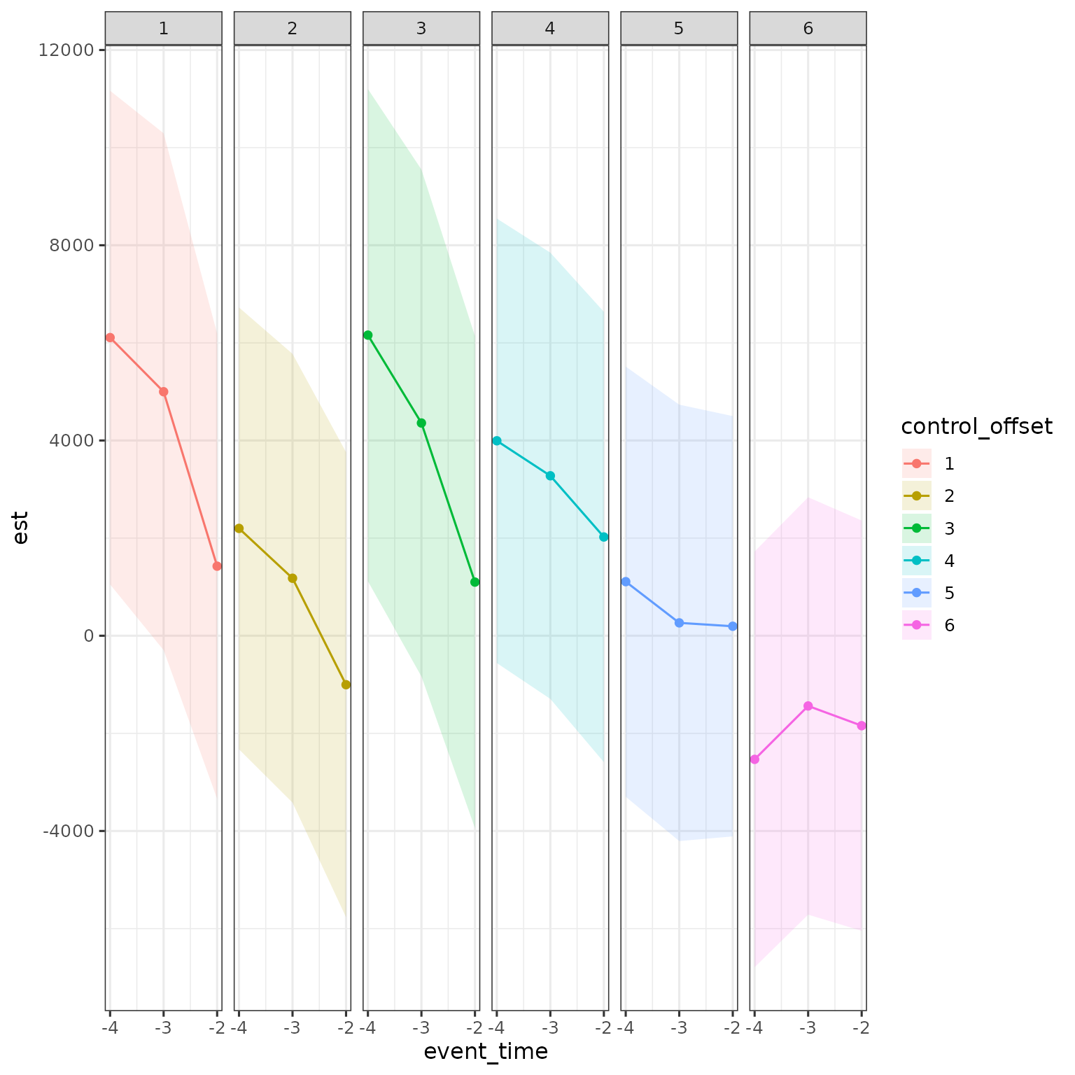

Although this would be hard to look at, we can put all control offsets on same plot.

res |> 
  filter(d == 25,
         a < d, 
         estimand == "ATE",
         method == "DID_Female") |> 
  mutate(control_offset = dp - d, 
         control_offset = factor(control_offset)) |> 
  ggplot(aes(x = event_time, y = est, ymin = ci_l, ymax = ci_h, color = control_offset, fill = control_offset)) +
  geom_ribbon(alpha = .15, color = NA) + geom_point() + geom_line() + 
  scale_x_continuous(breaks = -4:-2)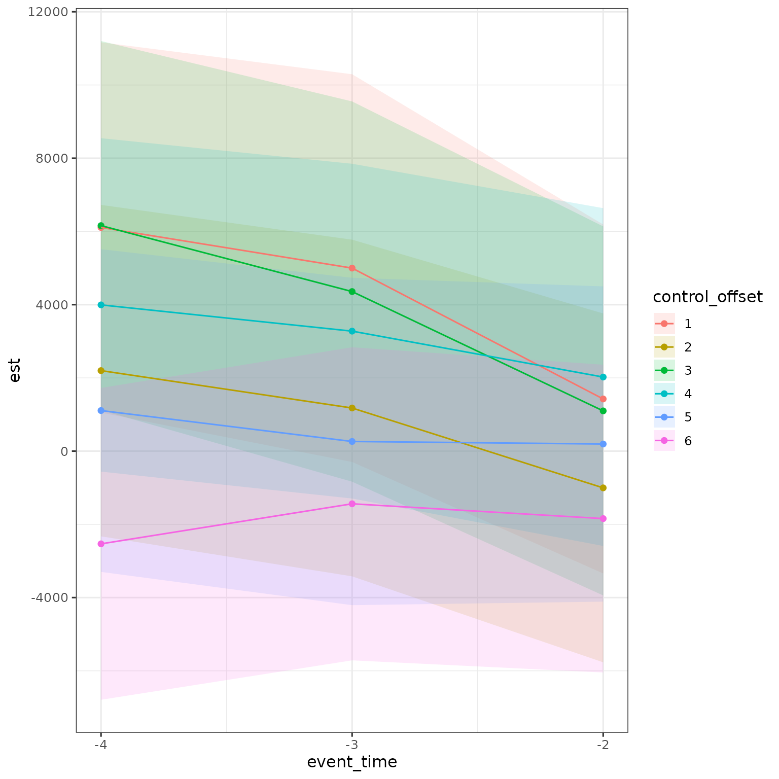

Can do this for multiple treatment groups at same time

res |> 
  filter(a < d, 
         estimand == "ATE",
         method == "DID_Female") |> 
  mutate(control_offset = dp - d, 
         control_offset = factor(control_offset)) |> 
  ggplot(aes(x = event_time, y = est, ymin = ci_l, ymax = ci_h, color = control_offset, fill = control_offset)) +
  geom_ribbon(alpha = .15, color = NA) + geom_point() + geom_line() + 
  scale_x_continuous(breaks = -4:-2) + 
  facet_grid(cols = vars(d))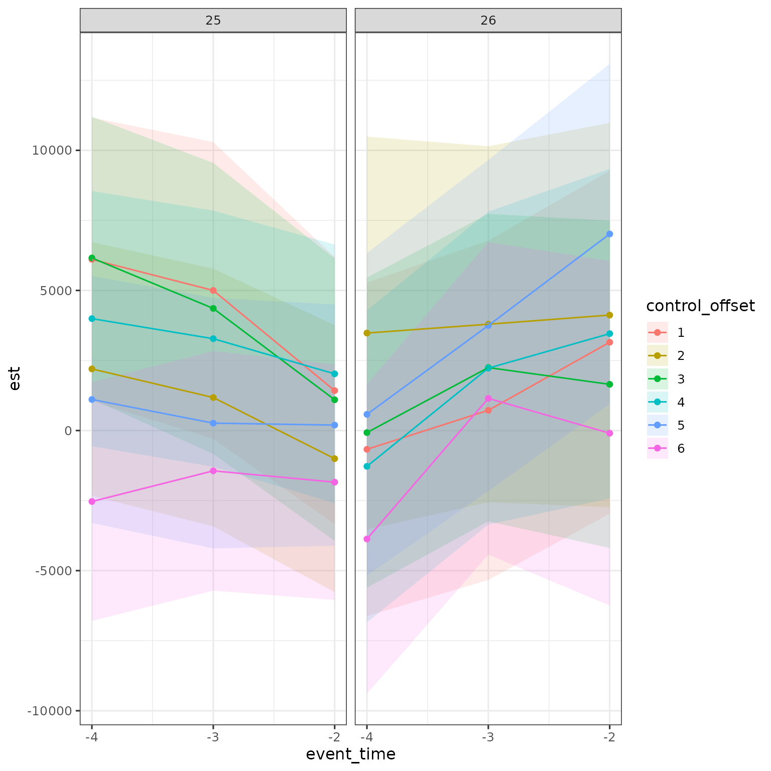

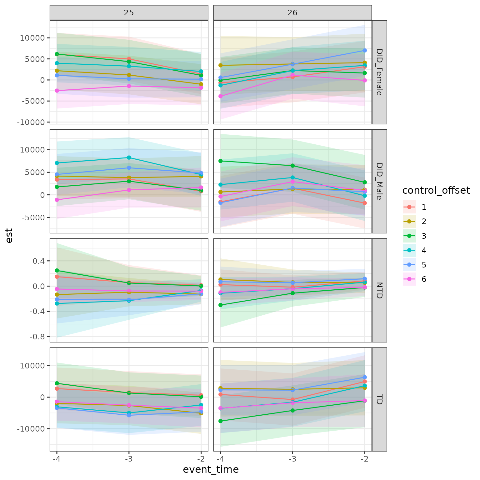
Finally, can do this for all methods.

res |> 
  filter(a < d, 
         estimand == "ATE" & (method == "DID_Female" | method == "DID_Male" | method == "TD") |
           estimand == "theta" & method == "NTD") |> 
  mutate(control_offset = dp - d, 
         control_offset = factor(control_offset)) |> 
  ggplot(aes(x = event_time, y = est, ymin = ci_l, ymax = ci_h, color = control_offset, fill = control_offset)) +
  geom_ribbon(alpha = .15, color = NA) + geom_point() + geom_line() + 
  scale_x_continuous(breaks = -4:-2) + 
  facet_grid(cols = vars(d), rows = vars(method), scales = "free")