DID-estimation • childpen

Overview

The aim of this vignette is show how to estimate DID using closest-not-yet-treated control groups using childpen.

Simulate data

The package has a built in simulation function to draw data resembling child penalty studies.

library(childpen)

N <- 20000
data <- simulate_data(n_individuals = N)
data |> tibble()
#> # A tibble: 420,000 × 6
#>       id female   age     D   Y_inf       Y
#>    <int>  <int> <int> <int>   <dbl>   <dbl>
#>  1     1      1    20    37   4455.   4455.
#>  2     1      1    21    37   7057.   7057.
#>  3     1      1    22    37  15138.  15138.
#>  4     1      1    23    37  31188.  31188.
#>  5     1      1    24    37  26199.  26199.
#>  6     1      1    25    37  45635.  45635.
#>  7     1      1    26    37  46719.  46719.
#>  8     1      1    27    37  39892.  39892.
#>  9     1      1    28    37 127141. 127141.
#> 10     1      1    29    37 109342. 109342.
#> # ℹ 419,990 more rows

Multiple treatment group analysis

We will now do the main heavy lifting. Say you want to estimate DID with closest-not-yet-treated control groups. This will be many $2\times2$ s. childpen easily allows it using the wrapper function below, multiple_treatment_group_analysis(). Note that the column names of the data are the same as the default for the function, so no need to input explicitly.

res = multiple_treatment_group_analysis(data = data,
                                  treatment_groups = 25:30, # which treatment groups to run in the analysis
                                  periods_post = 5, # estimate results for post periods 0:5
                                  periods_pre = NULL, # estimate pre-trend diagnostics, set to NULL to omit from estimation
                                  max_age = 40, # dont estimate results if age is above 40
                                  min_age = 20, # dont estimate results if age is below 20
                                  pre = 1, # use 1 period before treatment, can make further away if anticipation is conern
                                  verbose = FALSE # set to TRUE to output progress (i like to time loops) set to FALSE to omit messages
                                  )

Only DID, plot post-treatment results

The above function outputs results for all estimation methods discussed in the paper. Let save only DID results, and graph them. For benchmarking, I also add to the plots the mean observed earnings from the raw data.

obs_tidy = data |> 
  mutate(event_time = age - D) |> 
  rename(d = D) |> 
  group_by(female, d, event_time) |> 
  summarize(est = mean(Y)) |> 
  mutate(estimand = "APO", method = "Observed") |> 
  filter(event_time %in% -3:5, d %in% 25:30)

plot_data = res |> 
  filter(method %in% c("DID_Female", "DID_Male")) |> 
  mutate(female = ifelse(method == "DID_Female", 1, 0)) |> 
  select(d, event_time, estimand, female, est, ci_l, ci_h) |> 
  mutate(method = "DID")

plot_data = plot_data |> 
  dplyr::bind_rows(obs_tidy)

plot_data |> 
  filter(female == 1) |> 
  ggplot(aes(x = event_time, y = est, ymin = ci_l, ymax = ci_h, color = method, fill = method)) + 
  geom_ribbon(color = NA, alpha = .2) +
  geom_point() + geom_line() + 
  facet_grid(cols = vars(d), rows = vars(estimand), scales = "free") + 
  labs(x = "Event Time", y = "Estimate +/- 95% CI", color = "Method", fill = "Method") + 
  theme(legend.position = "bottom")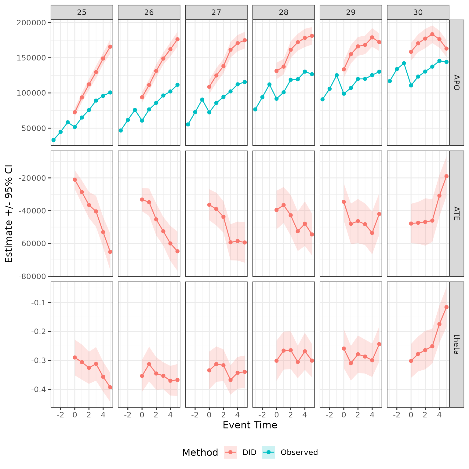

Compare to real effects in the simulation

The simulation offers also potential outcomes so we can see effect: Null for fathers and 30% decline with some constant recovery for mothers.

PO_tidy = data |> 
  mutate(event_time = age - D) |> 
  rename(d = D) |> 
  group_by(female, d, event_time) |> 
  summarize(APO_obs = mean(Y), APO = mean(Y_inf)) |> 
  mutate(ATE = APO_obs - APO, 
         theta = ATE / APO) |> 
  filter(event_time %in% 0:5, d %in% 25:30) |> 
  select(-APO_obs) |> 
  pivot_longer(
    !c(female, d, event_time), names_to = "estimand", values_to = "est"
  ) |> 
  mutate(method = "Truth")

plot_data = plot_data |> 
  dplyr::bind_rows(PO_tidy)

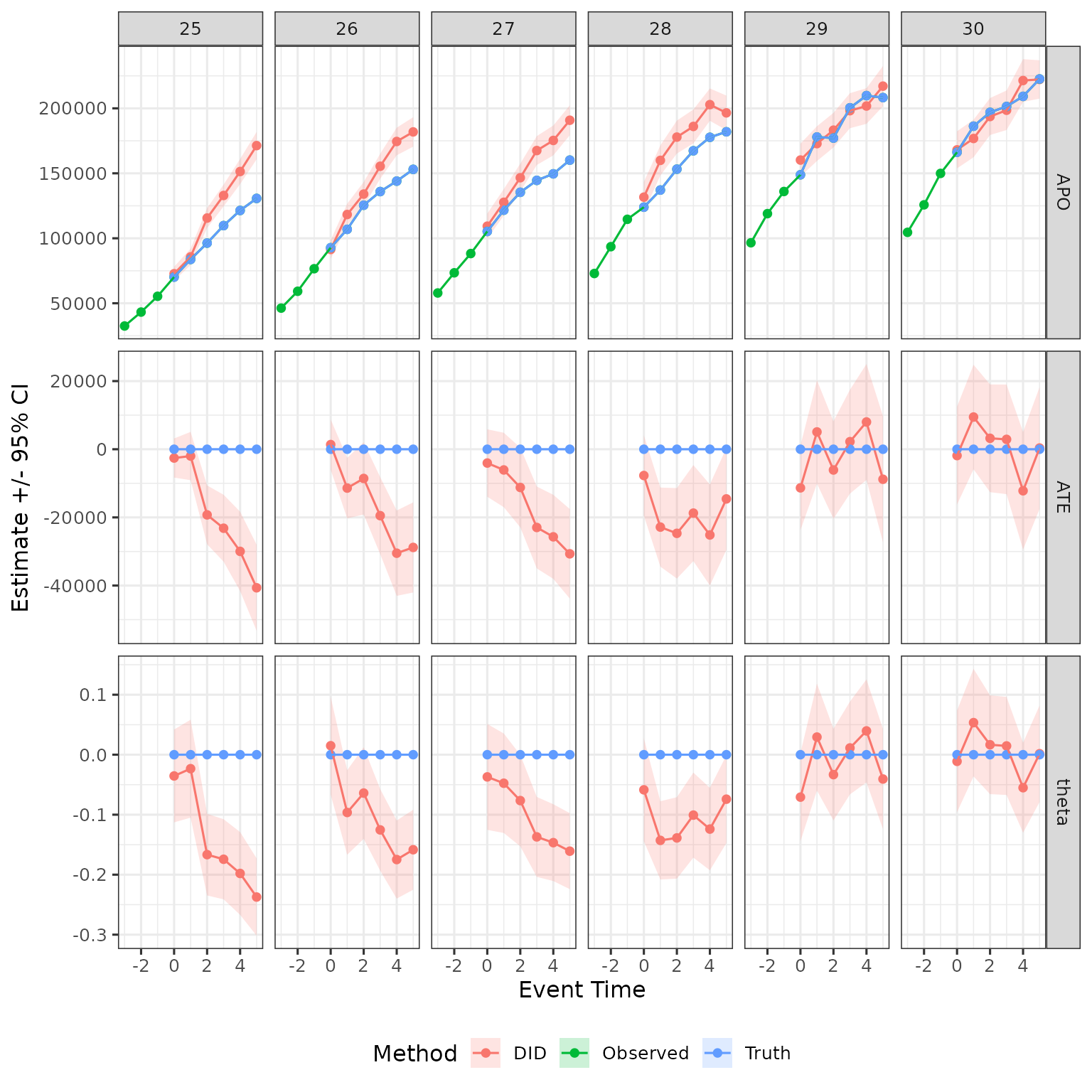
plot_data |> 
  filter(female == 1) |> 
  ggplot(aes(x = event_time, y = est, ymin = ci_l, ymax = ci_h, color = method, fill = method)) + 
  geom_ribbon(color = NA, alpha = .2) +
  geom_point() + geom_line() + 
  facet_grid(cols = vars(d), rows = vars(estimand), scales = "free") + 
  labs(x = "Event Time", y = "Estimate +/- 95% CI", color = "Method", fill = "Method") + 
  theme(legend.position = "bottom")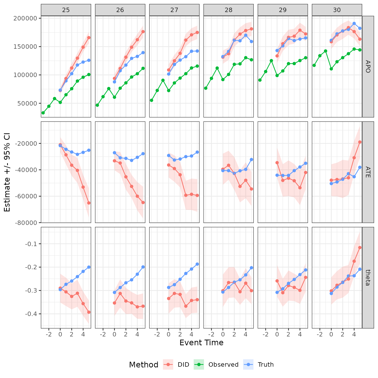

The intuition for this result, discussed in the paper, is that later treatment groups are positively selected compared to earlier treatment groups, and hence DID is overstating treatment effects for those groups.

For completness, show for men as well

plot_data |> 
  filter(female == 0) |> 
  ggplot(aes(x = event_time, y = est, ymin = ci_l, ymax = ci_h, color = method, fill = method)) + 
  geom_ribbon(color = NA, alpha = .2) +
  geom_point() + geom_line() + 
  facet_grid(cols = vars(d), rows = vars(estimand), scales = "free") + 
  labs(x = "Event Time", y = "Estimate +/- 95% CI", color = "Method", fill = "Method") + 
  theme(legend.position = "bottom")