Estimation

Notation. For symbol definitions, see the notation vignette.

Overview

childpen provides five estimators for the child penalty in earnings: DID_Female, DID_Male, TD, NTD_Conv, and NTD_New. All five are computed jointly by a single call to multiple_treatment_group_analysis(), which returns one row per treatment group $\times$ event time $\times$ estimand $\times$ method combination.

The estimators differ in what they target:

• DID_Female / DID_Male — gender-specific average treatment effects, using the closest not-yet-treated group as a control.
• TD — the gender gap in treatment effects (levels), i.e. ATE(female) − ATE(male).
• NTD_Conv — the conventional child penalty: the gender gap in normalised effects, $\theta_f - \theta_m$.
• NTD_New — the effect of parenthood on the gender earnings ratio $\rho$, denoted $\Delta\rho$.

Simulate data and run estimation

library(childpen)

data <- simulate_data(n_individuals = 2000, treatment_groups = 24:28)
head(data)
#>   id female age  D     Y
#> 1  1      1  20 24 40644
#> 2  1      1  21 24 36525
#> 3  1      1  22 24 39328
#> 4  1      1  23 24 34391
#> 5  1      1  24 24 46404
#> 6  1      1  25 24 46885

res <- multiple_treatment_group_analysis(
  data            = data,
  treatment_groups = 24:25,
  periods_post    = 2,
  periods_pre     = NULL,
  verbose         = FALSE
)

The data contain individuals with first birth ages ranging from 24 to 28. We analyse the two earliest groups (d = 24 and d = 25) over two post-birth periods. Groups with d ∈ {26, 27, 28} serve as not-yet-treated controls: for d = 24 at event time 2 (age 26) the control is d′ = 27; for d = 25 at event time 2 (age 27) the control is d′ = 28.

DID

DID estimates gender-specific effects using the closest not-yet-treated control group. For treatment group $d$ and target age $a$, the control group is $d^\prime = a + 1$. The DID counterfactual potential outcome is

$$\delta_{\mathrm{APO}}(g,d,d^\prime,a)=\mathbb{E}[Y_{d-1}\mid G=g, D=d]+\mathbb{E}[Y_a-Y_{d-1}\mid G=g, D=d^\prime]$$

and the DID ATE and normalised effect are

$$\delta_{\mathrm{ATE}}(g,d,d^\prime,a)=\mathbb{E}[Y_a\mid G=g, D=d]-\delta_{\mathrm{APO}}(g,d,d^\prime,a), \qquad \delta_{\theta}=\delta_{\mathrm{ATE}}/\delta_{\mathrm{APO}}.$$

When to use DID_Female / DID_Male: use these when you want gender-specific effect trajectories — for example, to plot the event-study path for women and men separately before computing any gap measure.

res |>
  filter(method %in% c("DID_Female", "DID_Male"),
         d %in% 24:25,
         event_time %in% 0:2) |>
  ggplot(aes(x = event_time, y = est, ymin = ci_l, ymax = ci_h,
             color = method, fill = method)) +
  geom_ribbon(color = NA, alpha = 0.2) +
  geom_point() + geom_line() +
  facet_grid(cols = vars(d), rows = vars(estimand), scales = "free") +
  labs(x = "Event Time", y = "Estimate +/- 95% CI",
       color = "Estimator", fill = "Estimator",
       title = "DID estimates by gender and treatment group") +
  theme(legend.position = "bottom")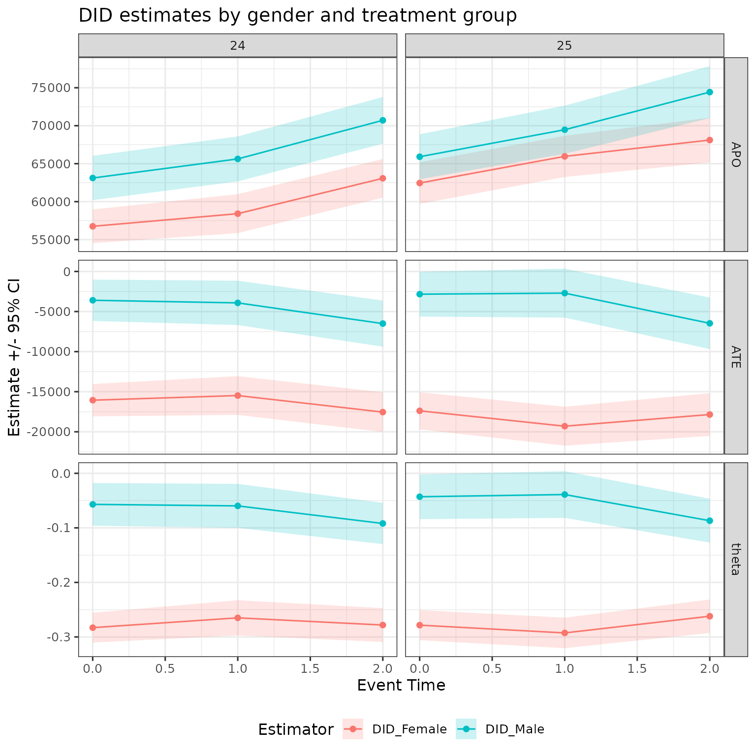

TD

TD estimates the gender gap in treatment effects in levels:

$$\mathrm{TD}(d, d^\prime, a) = \delta_{\mathrm{ATE}}(f, d, d^\prime, a) - \delta_{\mathrm{ATE}}(m, d, d^\prime, a).$$

When to use TD: use TD when your research question is about the absolute earnings gap attributable to parenthood — for example, how many currency units more does parenthood reduce female earnings than male earnings.

res |>
  filter(method == "TD",
         d %in% 24:25,
         event_time %in% 0:2) |>
  ggplot(aes(x = event_time, y = est, ymin = ci_l, ymax = ci_h)) +
  geom_ribbon(color = NA, alpha = 0.2, fill = "steelblue") +
  geom_point(color = "steelblue") + geom_line(color = "steelblue") +
  facet_grid(cols = vars(d), rows = vars(estimand), scales = "free") +
  labs(x = "Event Time", y = "Estimate +/- 95% CI",
       title = "TD: ATE(female) - ATE(male)") +
  theme(legend.position = "bottom")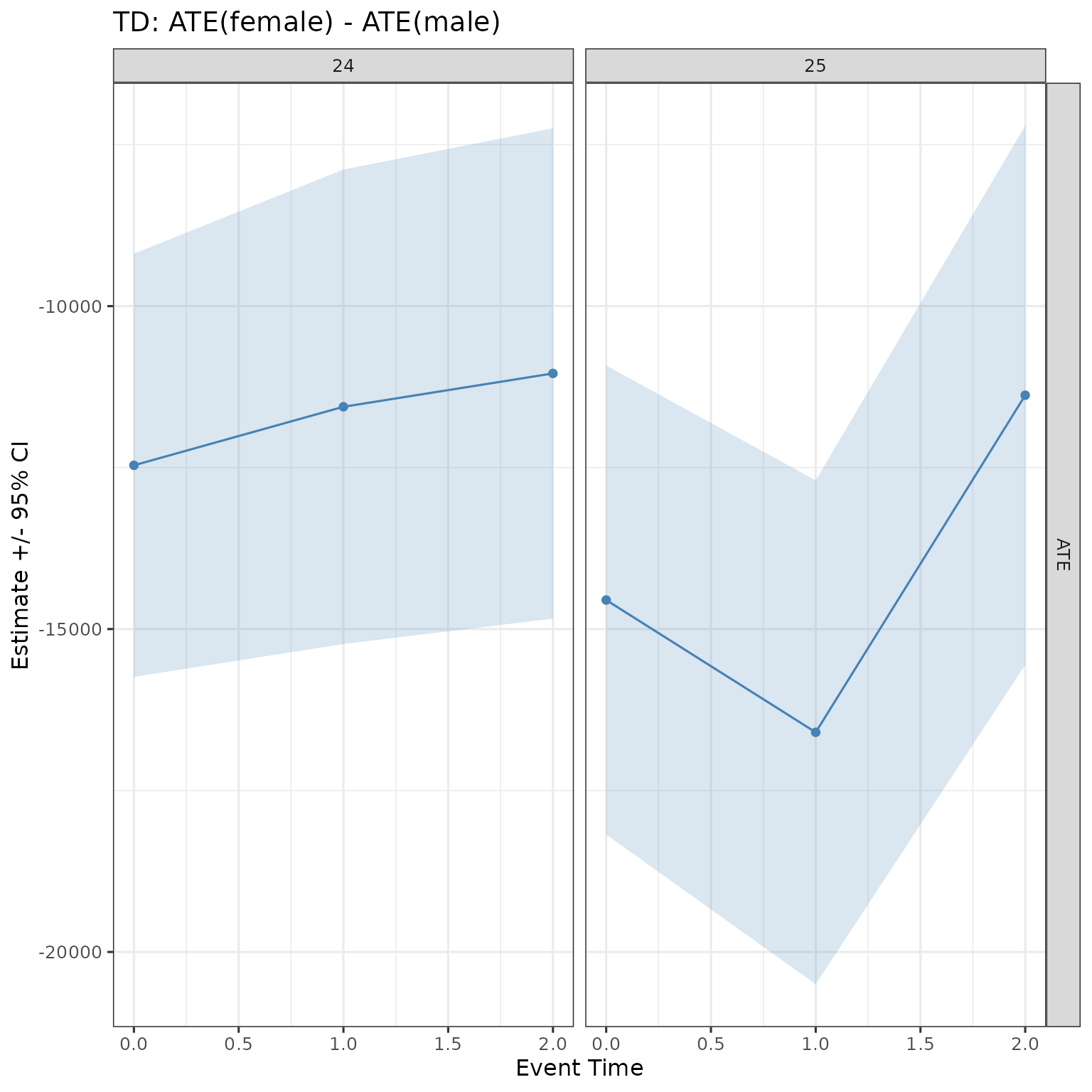

NTD

NTD produces two estimands that measure the gender gap in normalised terms.

NTD_Conv is the gap in normalised effects — the conventional child penalty:

$$\mathrm{NTD\_Conv}(d, d^\prime, a) = \delta_{\theta}(f, d, d^\prime, a) - \delta_{\theta}(m, d, d^\prime, a).$$

NTD_New measures the effect of parenthood on the gender earnings ratio $\rho$:

$$\mathrm{NTD\_New}(d, d^\prime, a) = \frac{\mathbb{E}[Y_a \mid f, D=d]}{\mathbb{E}[Y_a \mid m, D=d]} - \frac{\delta_{\mathrm{APO}}(f, d, d^\prime, a)}{\delta_{\mathrm{APO}}(m, d, d^\prime, a)} = \Delta\rho.$$

When to use NTD_Conv vs NTD_New: NTD_Conv normalises each gender’s ATE by its own pre-birth earnings level, so it is comparable across groups with different baseline earnings. NTD_New instead asks how much the ratio of female-to-male earnings changes because of parenthood, making it directly interpretable as a change in the gender earnings ratio.

NTD_Conv

res |>
  filter(method == "NTD_Conv",
         d %in% 24:25,
         event_time %in% 0:2) |>
  ggplot(aes(x = event_time, y = est, ymin = ci_l, ymax = ci_h)) +
  geom_ribbon(color = NA, alpha = 0.2, fill = "darkorange") +
  geom_point(color = "darkorange") + geom_line(color = "darkorange") +
  facet_grid(cols = vars(d), rows = vars(estimand), scales = "free") +
  labs(x = "Event Time", y = "Estimate +/- 95% CI",
       title = expression(paste("NTD_Conv: ", theta[f], " - ", theta[m]))) +
  theme(legend.position = "bottom")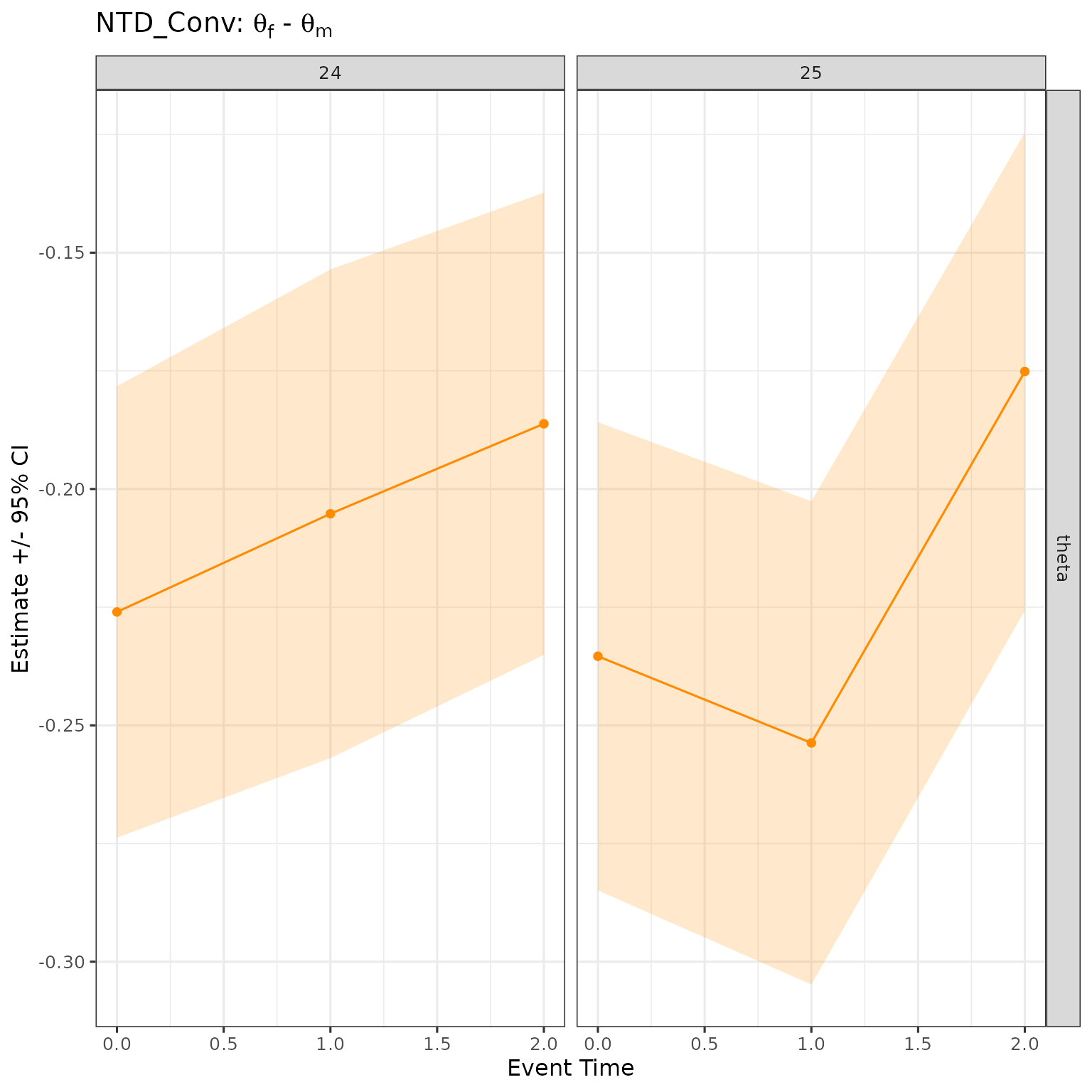

NTD_New

res |>
  filter(method == "NTD_New",
         d %in% 24:25,
         event_time %in% 0:2) |>
  ggplot(aes(x = event_time, y = est, ymin = ci_l, ymax = ci_h)) +
  geom_ribbon(color = NA, alpha = 0.2, fill = "darkgreen") +
  geom_point(color = "darkgreen") + geom_line(color = "darkgreen") +
  facet_grid(cols = vars(d), rows = vars(estimand), scales = "free") +
  labs(x = "Event Time", y = "Estimate +/- 95% CI",
       title = expression(paste("NTD_New: ", Delta, rho,
                                " (effect on gender earnings ratio)"))) +
  theme(legend.position = "bottom")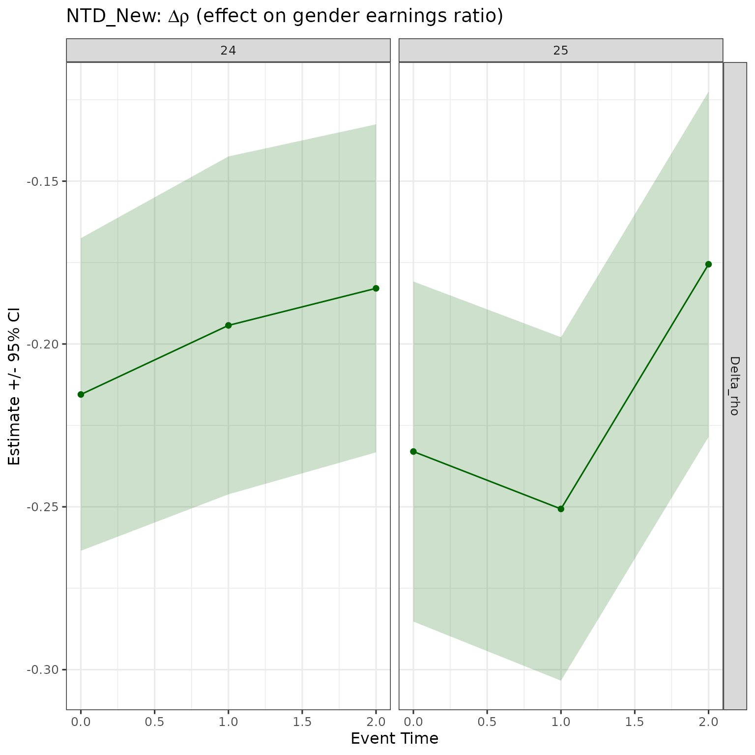

Validation tests

For a discussion of pre-trends tests and other validation checks appropriate for this estimator family, see the validation tests vignette.