aggregate-estimands • childpen

Notation. For symbol definitions, see the notation vignette.

Overview

multiple_treatment_group_analysis() estimates child-penalty effects separately for each treatment group $d$ (age at first birth). Because groups differ in their baseline earnings, age composition, and selection, a single group’s estimate is not directly comparable to another’s. aggregate_estimands() collapses the group-specific estimates into a single number per event time, answering the question: what is the average effect across the distribution of first-birth ages?

Three aggregate estimands are available:

avg_of_ratios ( $\theta_{\text{Agg},1}$ ): weighted average of each group’s normalized effect $\theta(g,d,d+e)$ . Formally, $\theta_{\text{Agg},1}(g,e) = \sum_d w_d \cdot \theta(g,d,d+e)$ , where $w_d$ are population weights normalised to sum to one. Preferred because normalization happens within each group before aggregation, so baseline differences do not inflate the average.
ratio_of_avgs ( $\theta_{\text{Agg},2}$ ): ratio of the weighted-average ATE to the weighted-average APO. Formally, $\theta_{\text{Agg},2}(g,e) = \sum_d w_d \cdot \text{ATE}(g,d,d+e) \;/\; \sum_d w_d \cdot \text{APO}(g,d,d+e)$ . This implicitly up-weights high-earning groups (their larger APO contributes proportionally more to the pooled denominator), so it differs from $\theta_{\text{Agg},1}$ when earnings vary across groups.
gender_ineq ( $\Delta\rho_{\text{Agg}}$ ): weighted average of NTD_New $\Delta\rho$ estimates — the aggregate gender-inequality penalty. Formally, $\Delta\rho_{\text{Agg}}(e) = \sum_d w_d \cdot \Delta\rho(d,d+e)$ .

Simulate and estimate

We simulate 2 000 individuals spanning treatment groups 24–30 (the extra groups serve as clean controls for the youngest treated cohorts), then analyse groups 24–27 with two post-treatment periods.

library(childpen)

data <- simulate_data(n_individuals = 2000, treatment_groups = 24:30)

res <- multiple_treatment_group_analysis(
  data             = data,
  treatment_groups = 24:27,
  periods_post     = 2,
  periods_pre      = NULL,
  verbose          = FALSE
)

Basic aggregation

Calling aggregate_estimands() with default arguments applies sample-proportion weights (weights = "sample"), where each treatment group is weighted by its share of the sample, as in Leventer (2025). Standard errors account for the estimation of these weights via the influence-function formula in the paper’s Appendix G. Pass weights = NULL for uniform weights.

agg <- aggregate_estimands(res)
head(agg)
#>   event_time estimand     method      agg_type       est        se n_groups
#> 1          0    theta DID_Female avg_of_ratios -0.246280 0.0110061        4
#> 2          1    theta DID_Female avg_of_ratios -0.283778 0.0100062        4
#> 3          2    theta DID_Female avg_of_ratios -0.274356 0.0098125        4
#> 4          0    theta   DID_Male avg_of_ratios -0.049832 0.0150746        4
#> 5          1    theta   DID_Male avg_of_ratios -0.046805 0.0137026        4
#> 6          2    theta   DID_Male avg_of_ratios -0.052369 0.0128336        4
#>        ci_l      ci_h
#> 1 -0.267851 -0.224708
#> 2 -0.303390 -0.264166
#> 3 -0.293589 -0.255124
#> 4 -0.079378 -0.020285
#> 5 -0.073662 -0.019947
#> 6 -0.077523 -0.027215

The output has one row per event_time × estimand × method × agg_type combination. The n_groups column records how many treatment groups contributed — useful for spotting cells where edge-of-sample groups drop out due to max_age/min_age bounds.

Plot aggregate results

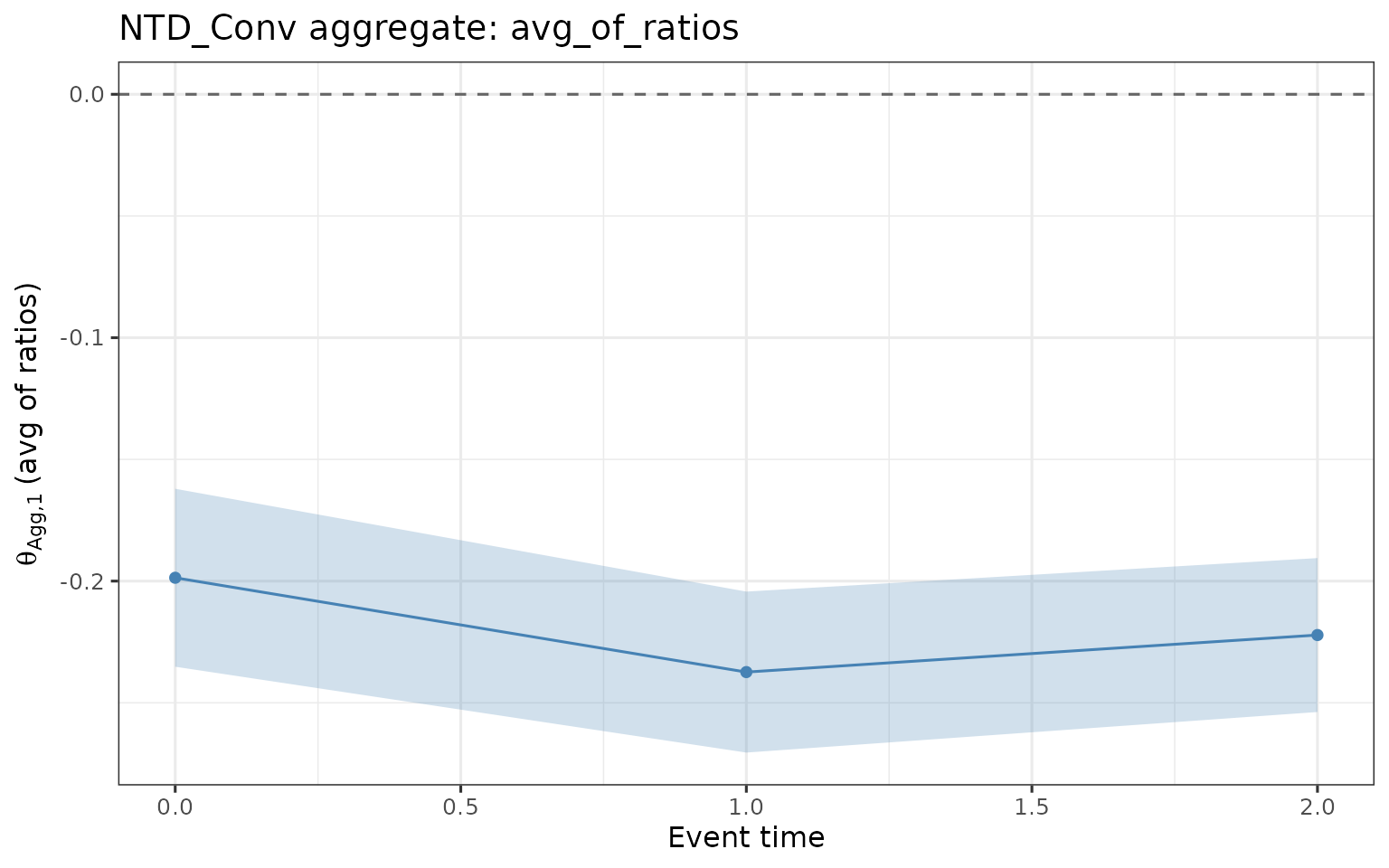
Plot the avg_of_ratios aggregate for the NTD_Conv method across event times, with 95% confidence ribbons.

agg |>
  filter(agg_type == "avg_of_ratios", method == "NTD_Conv", estimand == "theta") |>
  ggplot(aes(x = event_time, y = est, ymin = ci_l, ymax = ci_h)) +
  geom_ribbon(fill = "steelblue", alpha = 0.25, color = NA) +
  geom_line(color = "steelblue") +
  geom_point(color = "steelblue") +
  geom_hline(yintercept = 0, linetype = "dashed", color = "grey40") +
  labs(
    x     = "Event time",
    y     = expression(theta[Agg * "," * 1] ~ "(avg of ratios)"),
    title = "NTD_Conv aggregate: avg_of_ratios"
  )

Compare aggregation types

avg_of_ratios and ratio_of_avgs answer the same underlying question but weight groups differently. When high first-birth-age groups have higher counterfactual earnings than low first-birth-age groups, ratio_of_avgs assigns them more weight (the APO enters the denominator for each group before the ratio is formed across groups). The two estimands therefore diverge whenever earnings are heterogeneous across groups.

agg |>
  filter(
    agg_type %in% c("avg_of_ratios", "ratio_of_avgs"),
    method   == "DID_Female",
    estimand == "theta"
  ) |>
  ggplot(aes(
    x     = event_time,
    y     = est,
    ymin  = ci_l,
    ymax  = ci_h,
    color = agg_type,
    fill  = agg_type
  )) +
  geom_ribbon(alpha = 0.2, color = NA) +
  geom_line() +
  geom_point() +
  geom_hline(yintercept = 0, linetype = "dashed", color = "grey40") +
  labs(
    x     = "Event time",
    y     = expression(theta ~ "estimate"),
    title = "DID_Female: avg_of_ratios vs ratio_of_avgs",
    color = "Aggregation type",
    fill  = "Aggregation type"
  ) +
  theme(legend.position = "bottom")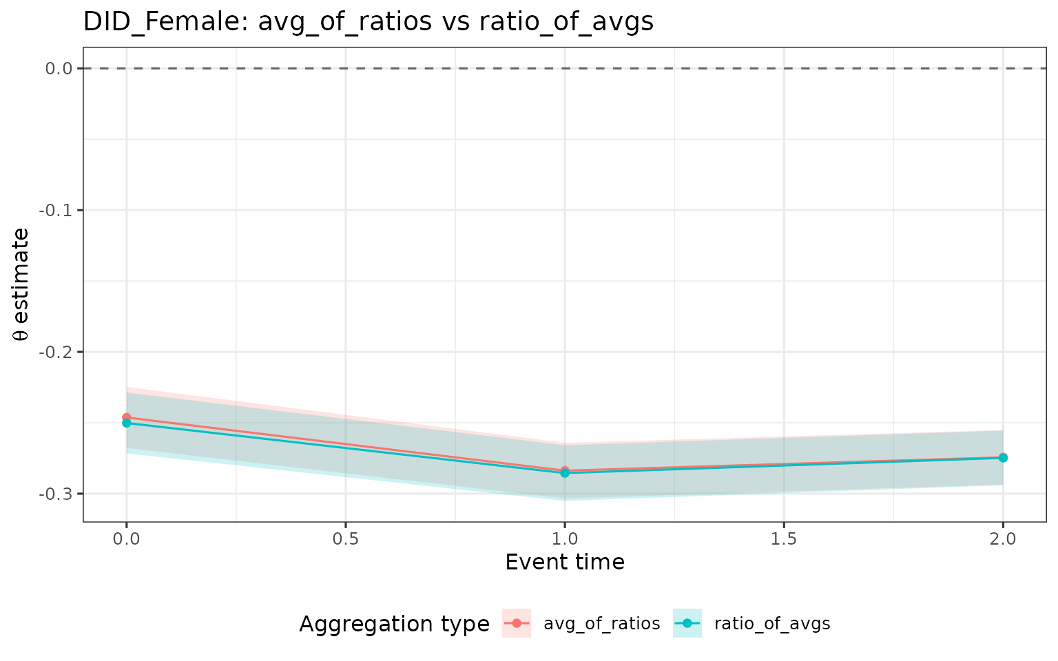

If the two lines are similar, earnings are approximately homogeneous across groups. Divergence is a sign that the treatment-group distribution interacts with baseline earnings levels, and the researcher must decide which weighting regime is more policy-relevant.

Custom weights

By default treatment groups are weighted by their sample proportions. Researchers may instead want to weight groups by their empirical share in a target population. Below we contrast two stylized distributions:

Right-skewed (mimicking the US): most first births concentrate at younger ages.
Left-skewed (mimicking Southern Europe): most first births concentrate at older ages.

groups <- as.character(24:27)

# Right-skewed: more weight on younger groups
w_us <- setNames(c(0.40, 0.30, 0.20, 0.10), groups)

# Left-skewed: more weight on older groups
w_se <- setNames(c(0.10, 0.20, 0.30, 0.40), groups)

agg_us <- aggregate_estimands(res, weights = w_us)
agg_se <- aggregate_estimands(res, weights = w_se)

bind_rows(
  mutate(agg_us, population = "US (right-skewed)"),
  mutate(agg_se, population = "Southern Europe (left-skewed)")
) |>
  filter(
    agg_type == "avg_of_ratios",
    method   == "NTD_Conv",
    estimand == "theta"
  ) |>
  ggplot(aes(
    x     = event_time,
    y     = est,
    ymin  = ci_l,
    ymax  = ci_h,
    color = population,
    fill  = population
  )) +
  geom_ribbon(alpha = 0.2, color = NA) +
  geom_line() +
  geom_point() +
  geom_hline(yintercept = 0, linetype = "dashed", color = "grey40") +
  labs(
    x     = "Event time",
    y     = expression(theta[Agg * "," * 1]),
    title = "Aggregate NTD_Conv estimate under different first-birth distributions",
    color = "Population weights",
    fill  = "Population weights"
  ) +
  theme(legend.position = "bottom")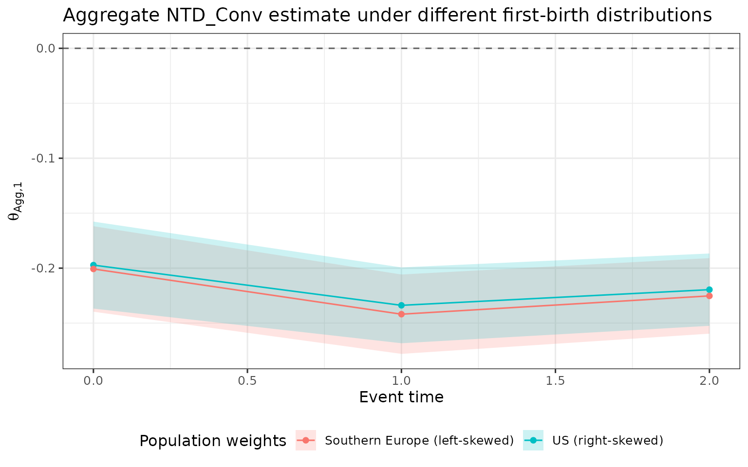

When younger groups bear larger penalties than older groups (or vice versa), the choice of weight vector shifts the aggregate estimate. Reporting both provides a sensitivity check on how much the aggregate depends on the first-birth distribution.

Gender inequality aggregate

The gender_ineq aggregate ( $\Delta\rho_{\text{Agg}}$ ) is the weighted average of NTD_New $\Delta\rho$ estimates across treatment groups. It measures how parenthood affects the female-to-male earnings ratio: negative values indicate that mothers bear a larger proportional penalty — the female-to-male earnings ratio is lower post-birth than the counterfactual ratio.

agg |>
  filter(agg_type == "gender_ineq", estimand == "Delta_rho", method == "NTD_New") |>
  ggplot(aes(x = event_time, y = est, ymin = ci_l, ymax = ci_h)) +
  geom_ribbon(fill = "tomato", alpha = 0.25, color = NA) +
  geom_line(color = "tomato") +
  geom_point(color = "tomato") +
  geom_hline(yintercept = 0, linetype = "dashed", color = "grey40") +
  labs(
    x     = "Event time",
    y     = expression(Delta * rho[Agg]),
    title = "Gender inequality aggregate (NTD_New, avg of ratios)"
  )

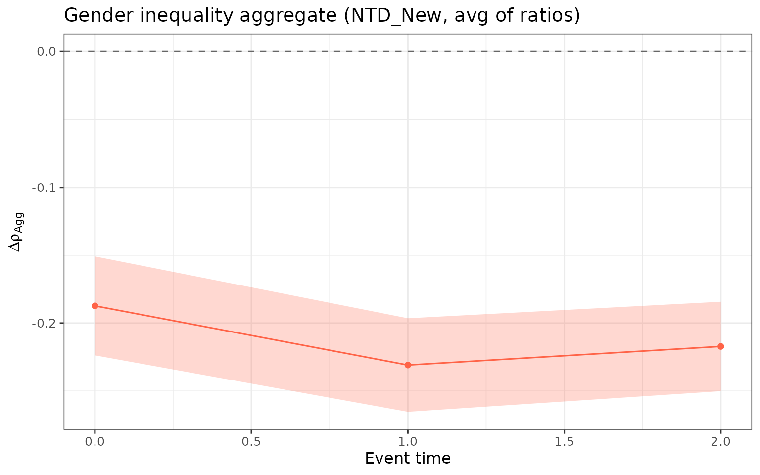
A flat, negative profile indicates a persistent parenthood-driven gender gap; values closer to zero at later event times suggest the gap narrows as parents age away from the birth event.